Documentation

How to use PhysioMEA:

Load, Present, and Save Raw Data

1. Run PhysioMEA_GUI.m. To load a single file, press the button next to “Record file name”, select file type – supported file types are .mcd (default) and .h5 recorded from Multi-Channel Systems recording device. To load consecutive recorded files of the same experiment, first choose file type next to “Data type” – supported file types are .mcd (default) and .h5, and then, press the button next to “Folder name” and choose a data folder to load all files from this folder of the chosen type. The loaded files will appear on the list next to “Files”. To load single file, also use the Main Manu, press “File” and then, “Open data file” or Ctrl+O.
2. Name the experiment analysis project on the textbox next to “Experiment name”. The name should start with a letter and should not include spaces or special characters.
3. Electrode spacing value (100 or 200 micrometers) is loaded according to the value stored on the loaded file, resulted in from the MEA plate model defined on the recording data software.
4. On “Channels” tab, the recorded channels, which appear on the loaded files, are shown. By pressing on channel number on the “On” Channel tab located in the “Channels” tab, all raw data from this channel are plotted on the “Data” tab (for multiple files loaded, the data from each channel is concatenated).
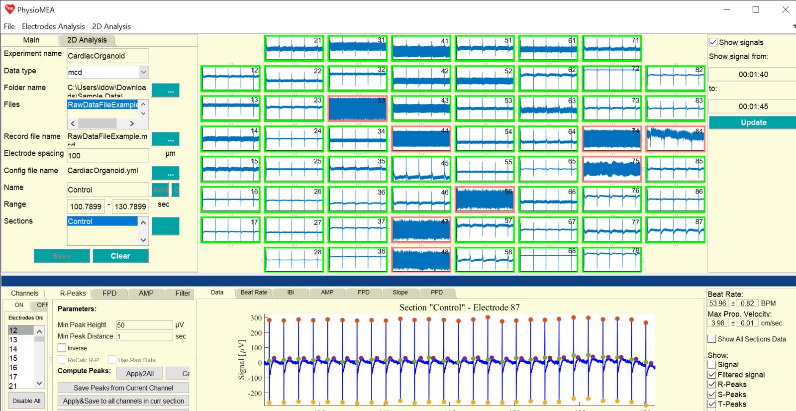
5. To plot data from all channels on the matrix of figures, which represent the MEA plate, define a range on the text boxes as hh:mm:ss or as a value in seconds, which will be automatically converted to such representation. Then, press on the “Update” button and tick the “Show signals” box: all 60 figures will present the raw data of the defined time range. To choose different range, change the time values to the desired range and press on the “Update” button.
6. This 60-figure presentation of signals can be used to inspect the raw data and define the high and low signal-to-noise ratio channels. As default, all channels considered as “On” and their figure marked with green rectangle. To switch a channel into “Off” mode, press on the figure (on the white background where there is no signal), the channel is switched to “Off” mode, and the color of the rectangle around it is changed into red. Data of the “Off” mode channels will be rejected for the next analysis process. Pressing on the “Disable All” on the “Channels” tab defined all channels as “Off”, and pressing on one of the figures makes is “On” again. This option can serve for mono-channel of low channel number analysis.
7. Next, to choose a time section for analysis, press on one of the channels on the “On” Channel tab located in the “Channels” tab. Define a name for the section on the textbox next to “Name”, define time range (in seconds) on the two textboxes (from and to), and press “Add”. Section’s name should not include special characters. A rectangle signing the time range appears on the figure located in the “Data” tab. By dragging the section’s rectangle, its range is changed on the textboxes. To add another section, name the section on the textbox next to “Name”, define time range (delete the written values on the textboxes next to “Range”), and press “Add” button. To delete a section, press on its name on the list next to “Sections”, and press “Del” button.
8. To load a previous saved section and “On” channel configuration, press the button next to the sections’ list, and load a section configuration .yml file.
9. Press “Save” button and choose path for the analysis folder on the displayed window. Then, raw data are saved by channel and section on the analysis folder, and analysis configuration and section configuration .yml files are created and saved in the same folder. Top save the analysis, also use the Main Manu, press “File” and then, “Save data per section” or Ctrl+S. To save only the section configuration .yml file, use the Main Manu, press “File” and then, “Save sections times” or Ctrl+T.
10. Press “Clear” button to clear the experiment analysis project.

Peak Detection and Biomarker Calculation

1. To perform peak detection, continue after saving raw data as explained above or load analysis by loading an analysis configuration .yml file: press on the button next to “Config file name” and choose an analysis configuration .yml file. To load analysis by analysis configuration .yml file, also use Main Manu, press “File” and then, “Load data per section” or Ctrl+D.
2. The raw data of the first section, which appears on the sections list next to “Sections”, and the first channel, which appears on the “On” Channel tab, located in the “Channels” tab, is presented on the “Data” tab. To present other section or channel data, press on the section name or channel name on the corresponding lists. The “Off” channels are listed in the “Off” tab in the “Channels” tab (their data are not saved).
3. To define filtration and peak detection parameters, use the “R-Peaks”, “FPD”, “AMP”, and “Filter” tabs: for R-peaks, on the “R-Peaks” tab define the minimum peak voltage in the textbox next to “Min Peak Height” (in micro-volts) and the minimum time interval between peaks in the textbox next to “Min Peak Distance” (in seconds). For low R-peaks and high S-peaks (in an absolute value) voltage, tick the box next to “inverse” to apply the R-peak detection algorithm on the S-peaks (for the inverted signal) and then, automatically find the adjacent R-peaks. For T-peaks, define the time interval after R-peaks to identify them on the two textboxes on the “FPD” tab below “Time interval to search after R-Peaks” (from and to, in seconds). For S-peaks, define to maximal time interval after R-peaks to identify them on the textbox below “Time interval search after R-Peaks” (in seconds). It is recommended that the minimum time interval after R-peaks to identify the T-peaks is equal of higher than the maximal time interval after R-peaks to identify the S-peaks.
4. Raw data filter includes a band-pass filter to eliminate noise outside the defined range, and application of a notch filter to suppress electrical interference. Define the band-pass filter frequency range by the textboxes next to “BPF – High Cutoff” and “BPF – Low Cutoff” (Hz) on the “Filter” Tab”. Typically, for European standard, choose 50 Hz, and for US standard, 60 Hz, on the list next to “Electrical Frequency” on the “Filter” tab.
5. Peak detection algorithms are applied on the filtered signal. To identify the R-, S-, and T-peaks according to the raw data, tick the “Use Raw Data” box on each tab (“R-Peaks”, “FPD”, and “AMP”).
6. To compute the filtered signal and detect the peaks, press on the “Calc” button next to “Compute Peaks”. In addition to the presented raw data (“Signal”) on the “Data” tab, the filtered signal (“Filtered signal”), R-, S-, and T-peaks, Maximal Slope (Slope), and Peak-to-Peak Duration (PPD) are presented. To remove to presentation of some of them, press the corresponding box.
7. To apply the same peak-detection parameters to all channels, press on the “Apply2All” button next to “Compute Peaks”.
8. To save filtered signal, peaks’, and biomarkers’ files, press on one of the three buttons: “Save Peaks from Current Channel” to calculate and save these data files of the current presented channel’s data of the chosen section; “Apply&Save to all channels in curr section” to calculate and save these data files of all channels of the chosen section; “Apply&Save to all channels in all section” to save these files of all channels and sections.
9. The calculated beat rate of each channel for each section, according to the calculated inter-beat intervals (and detected R-peaks), is presented under “Beat Rate” (in beat per minute, BPM) including its standard deviation. For more than one channel analyzed, the maximal propagation velocity per beat spreading through the electrode array of the MEA plate and calculated according to the maximal propagation period, is presented under “Max Prop. Velocity” (in centimeters to seconds, cm/sec), including its standard deviation.
10. On “Beat Rate” tab, a bar graph of the mean beat rate with its standard deviation is presented for the chosen channel of the chosen section. To add the graph the bar(s) of the other section(s), tick the “Show All Sections Data” box.
11. On “IBI”, “AMP”, “FPD”, “Slope”, and “PPD” tabs, the following figures are presented for the biomarkers derived from the chosen channel of the chosen section: the biomarker time series as function of time, a bar graph of the mean biomarker time series data with its standard deviation including a scatter of the biomarker time series data, and a histogram of the biomarker time series data as a percentage. To add the corresponding plot(s), bar(s), and histogram(s) of the other section(s), tick the “Show All Sections Data” box.
12. To save figures, use the Main Manu, press “File” and then, “Save figures” or Ctrl+F. On the opened window, tick the desired graphs to be saved, press “Save As”, and choose a folder to save in the figure files and a file type (e.g. fig, jpg, pdf, svg) or press “Cancel” to close the window.
13. To save mean biomarker data for each section and channel, use the Main Manu, press “Electrode Analysis” and then, “Save Analysis to Excel” or Ctrl+A, and choose a folder to save in the data file. A window states “The file [file path and name] was saved.” will be opened – press “OK” button on the window to continue.

Two-Dimensional (2D) Analysis

1. On “Main” tab, choose a section from the section list next to “Sections”.
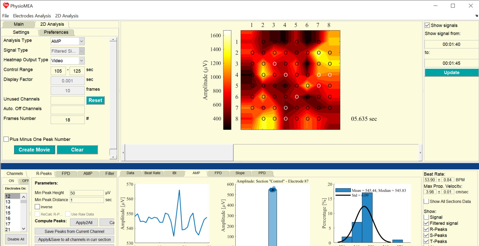
2. On “2D Analysis” tab, choose the analysis type from the list next to “Analysis Type”. For “Potential”, choose raw or filtered signal from the list next to “Signal Type”. For other analysis types, the 2D data is based on a calculated data (“Signal Propagation”) or saved biomarkers (“FPD”, “AMP”, “Slope”, and “PPD”), thus, signal type list is disabled.
3. On the list next to “Heatmap Output Type”, choose how to plot the frames of the 2D analysis: “Video” (consecutive frames one after the other), “Subplots” (a figure with subplots, which each represent one frame), “One Frame” (a single frame which is the average of all frames), “3D Video” (consecutive frames one after the other, each plotted as a 3D figure), “3D Frame” (a single frame which is the average of all frames, plotted as a 3D figure).
4. Define a time range (in seconds) from which to present the data on the two textboxes (from and to) next to “Range”. Chosen section’s name appears before the word “Range”.
5. For “Potential”, the maximal temporal resolution for 2D analysis is dependent on the sampling frequency, thus, 2D analysis can reach, for example, 10,000 frames in second for 10,000 Hz recording. To reduce the temporal resolution for the 2D analysis, define the desired 2D analysis temporal resolution on one of the two textboxes next to or below “Display Factor”: on the top textbox, define it as the time step for each frame (in seconds), and the corresponding frame number occurs in this duration, based on the sampling frequency, will be automatically calculated accordingly; alternatively, on the textbox below, define the frame number, based on the sampling frequency, to be considered as one frame for each frame of the 2D analysis (in frames, corresponding to samples of the signal), and the corresponding time step will be automatically calculated accordingly. To average the frames along each step instead of skipping them (according to the defined frame number), tick the box near “Calc Mean Frame Data”.
6. To choose channels to exclude from the 2D analysis (e.g. low signal-to-noise ratio identified after data saving earlier), double-click the desired channels to be excluded on the “On” Channel tab, located in the “Channels” tab, and these channel numbers will be removed from the “On” Channel tab and appear on the textbox next to “Unused Channels”. To cancel the exclusion of these channels, press on the “Reset” button next to the textbox that is next to “Unused Channels”.
7. For analysis types other than “Potential” – “Signal Propagation” or biomarkers (“FPD”, “AMP”, “Slope”, and “PPD”) – channels with different peak number than the majority of the channels are automatically considered as unused, and appear on the textbox next to “Auto. Off Channels”. To include channels with peak number that is higher or lower by only one peak, tick the box near “Plus Minus One Peak Number”.
8. Press “Create Movie” to plot the chosen 2D analysis type by the chosen heatmap output type. For “Video” or “3D Video”, a 2D figure with a scroll under it is presented, and by moving the scroll the figure and time stamp is updated. For “Subplots”, new window with corresponding subplots is opened. For “One Frame” or “3D Frame”, one figure is presented (with disabled scroll).
9. On the “Preferences” tab, the heatmap settings are defined: the list next to “Color Set” includes proposed heatmap color sets with automated default color set for each analysis type; the list next to “Expand Matrix Borders” offers options for matrix border expansion for 2D or 3D presentation including “with Nearest Values”, “With Zeros”, or without expansion (“No”); heatmap color scale number can be defined as an integer number on the textbox next to “Contours Number”; missing channels (off, unused, or automated off channels) are filled-in on the presented frames using a fill-in missing algorithm based on a moving average method with a window length that can be defined according to the integer number on the textbox next to “Filling-in Factor” (window length), and is applied to complete the spatial gaps; the color scale limits can be defined on the textboxes (from and to) next to “Level Limits”; electrode presentation on the plotted frames can be chosen according to the options on the list next to “Channel Circles”, including “On” (black circles for on channels and white for filled-in missing channels), “Values” (written values in black or white, respectively), “Off” (with no sign for the electrodes), or “Arrows” (directional arrows); time stamp is presented according to the box near “Time Counter” (appears when it is ticked).
10. Additionally, the “Preferences” tab also includes settings to save the 2D analysis as a video file: file format is chosen on the list next to “Video Type”, including “mp4” or “avi”; the frame rate is defined as an integer number on the textbox next to “Frame Rate” in frames per second (frame/sec).
11. To save a movie file, use the Main Manu, press “2D Analysis” and then, “Save movie” or Ctrl+M, and choose a folder to save in the video file. Alternatively, to save 2D analysis data including 3D matrix of frame data over time and video configuration settings, press “Save analysis data” or Ctrl+D – a .mat file stores the data will be save on the analysis folder, and a window states “The data was saved!” will be opened. Press “OK” button on the window to continue.
12. Use the Main Manu, press “File” and then, “Exit” or Ctrl+E to close the graphical user interface (GUI) window.

Beat Rate Variability Analysis

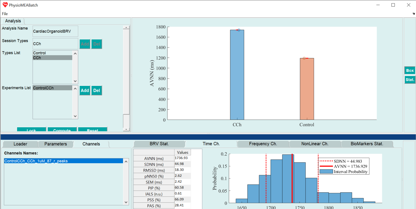
1. Run PhysioMEABatch_GUI.m. Name the Beat Rate Variability (BRV) analysis project on the textbox next to “Analysis name”. The name should not include special characters.
2. Define session types as experimental categories for the analysis (such as different drug concentrations or experimental conditions) by entering each session type’s name on the textbox next to “Session Types” and press “Add” button. The session type name appears on the list next to “Types List”. These names can be different that the sections names on the experiment analysis projects to be further loaded. To delete inserted session type, press it on the list and press “Del” button.
3. Load experiment analysis project analyzed with PhysioMEA module by pressing “Add” button next to the list located next to “Experiments List”. On the opened window, choose analysis configuration .yml file. To delete an inserted experiment analysis project, press in on the list and press “Del” button. When finished inserting session types and loading experiment analysis projects, press “Lock” button.
4. For each loaded experiment analysis project, press on its name on the experiment list, and then, on the “Loader” tab attribute between the session type in the “Types” (first) column on the table in the tab and the corresponding section of the loaded experiment analysis project. For that purpose, use the sections list derived from the experiment analysis project data on the “Sections” (second) column. On the “Channels” (third) column, choose channel for analysis from the channel list derived from the experiment analysis project data or choose “All” to choose analyzing all channels of this section. Repeat this step to all loaded experiment analysis projects on the experiment list.
5. Press “Compute” to run BRV analysis and choose a folder in which to save the analysis files.
6. BRV analysis is performed by PhysioZoo toolbox based on calculated R-peaks analyzed by PhysioMEA and by using BRV parameters of the default loaded configuration file presented on “Parameters” tab. Press the button next to “Config file name” to load different configuration file. Default BRV analysis in performed by analyzing full R-peak time series data derived from each channel, as the “Full Signal Length” button is chosen. Choose “Window Length” option to define different window length to divide each R-peak time series data into, by inserting the desired time length on the appeared textbox as hh:mm:ss.
7. On the “BRV Stat.” tab, BRV measures are listed (“Measures”, first column) together with their description (“Description”, second column). For each session type, the mean measures are presented as mean and standard deviation (according to the session type names, starting from the third column onwards, by the session type number). When pressing each line of the table, the corresponding BRV measure by session type is presented as bar graph, which each bar represents the mean BRV measure of all analyzed channels of the session type corresponding to all loaded experiment analysis projects. To save the presented bar graph, use the Main Manu, press “File” and then, “Save Main Figure” or Ctrl+M. Choose a folder to save in the figure file and a file type (e.g. fig, jpg, pdf, svg).
8. “BioMarkers Stat.” tab contains a table of biomarkers, their description, and their mean values together with their standard deviation for all session types (corresponding to the attributed sections of the loaded experiment analysis project).
9. On the “Channel” tab, the loaded channels are presented according to the chosen experiment on the experiment list and the chosen type corresponding to the section of the loaded experiment analysis project. By choosing channel name from the list, its BRV measures and figures are presented on: “Time Ch.” Tab, containing a mean time domain BRV measure table and inter-beat interval histogram; “Frequency Ch.” Tab, containing a mean frequency domain BRV measure table and graphs including the power spectral density as function of frequency (by clicking on “Log” button, y axis values are changed into the natural logarithm of these values, and by clicking on this button, which its text was changed into “Linear”, y axis values are back to their original values) and the natural logarithm of power spectral density as function of the natural logarithm of the frequency; “NonLinear Ch.” Tab, containing a mean non-linear BRV measure table, detrended fluctuation analysis graph, Poincare Plot, and Multi-Scale Entropy graph.
10. To save a BRV analysis project configuration .yml file, use the Main Manu, press “File” and then, “Save Analysis” or Ctrl+S. Choose folder on the displayed window to save the file in, and a window states “The data was saved!” will be opened. Press “OK” button on the window to continue.
11. To load a BRV analysis project configuration .yml file, use the Main Manu, press “File” and then, “Load Analysis” or Ctrl+O. Choose .yml file on the displayed window, and the BRV analysis project is loaded. Press “Compute” button to run BRV analysis and choose a folder in which to save the analysis files.
12. Press “Reset” button to clear the BRV analysis project.
13. Use the Main Manu, press “File” and then, “Exit” or Ctrl+E to close the graphical user interface (GUI) window.